Python package

This page shows some simple examples of using the planetmapper package in Python code. For more details, see the full API documentation.

For PlanetMapper to function, you will need to download a series of SPICE kernels containing the positions and orientations of the solar system bodies you are interested in. The code snippet below will download all the appropriate kernels needed for the examples on this page. For more details about SPICE kernels, including how to choose, download, and use them, see the SPICE kernel documentation page.

from planetmapper.kernel_downloader import download_urls
# This command will download ~2GB of data
# Note, the exact URLs in this example may not work if new kernel versions are published
download_urls(
    'https://naif.jpl.nasa.gov/pub/naif/generic_kernels/lsk/',
    'https://naif.jpl.nasa.gov/pub/naif/generic_kernels/pck/',
    'https://naif.jpl.nasa.gov/pub/naif/generic_kernels/spk/planets/de430.bsp',
    'https://naif.jpl.nasa.gov/pub/naif/generic_kernels/spk/satellites/jup365.bsp',
    'https://naif.jpl.nasa.gov/pub/naif/generic_kernels/spk/satellites/sat441.bsp',
    'https://naif.jpl.nasa.gov/pub/naif/generic_kernels/spk/satellites/ura111.bsp',
    'https://naif.jpl.nasa.gov/pub/naif/generic_kernels/spk/satellites/nep097.bsp',
    'https://naif.jpl.nasa.gov/pub/naif/HST/kernels/spk/',
)

Coordinate conversions

Coordinate conversions can easily be performed using functions such as planetmapper.Body.lonlat2radec() to calculate the sky coordinates corresponding to a planetographic longitude/latitude coordinate on the surface of the target.

This code shows an example of using some of the functions in planetmapper.Body to calculate information about observations of Jupiter from Venus:

import planetmapper

body = planetmapper.Body('jupiter', '2020-01-01', observer='venus')

coordinates = [(42, 0), (123, 45)]
for lon, lat in coordinates:
    print(f'\nlongitude = {lon}°, latitude = {lat}°')
    if body.test_if_lonlat_visible(lon, lat):
        ra, dec = body.lonlat2radec(lon, lat)
        print(f'  RA = {ra:.4f}°, Dec = {dec:.4f}°')
        if body.test_if_lonlat_illuminated(lon, lat):
            phase, incidence, emission = body.illumination_angles_from_lonlat(lon, lat)
            print(f'  phase angle: {phase:.2f}°')
            print(f'  incidence angle: {phase:.2f}°')
            print(f'  emission angle: {phase:.2f}°')
    else:
        print('  (Not visible)')

Hint

The main classes in PlanetMapper are subclasses of each other, with planetmapper.SpiceBase the parent class of planetmapper.Body which is the parent of planetmapper.BodyXY which is the parent of planetmapper.Observation.

In Python, any functions defined in a parent class are available in any subclasses, so for example, you can use planetmapper.Observation.lonlat2radec() exactly the same way as you can use planetmapper.Body.lonlat2radec().

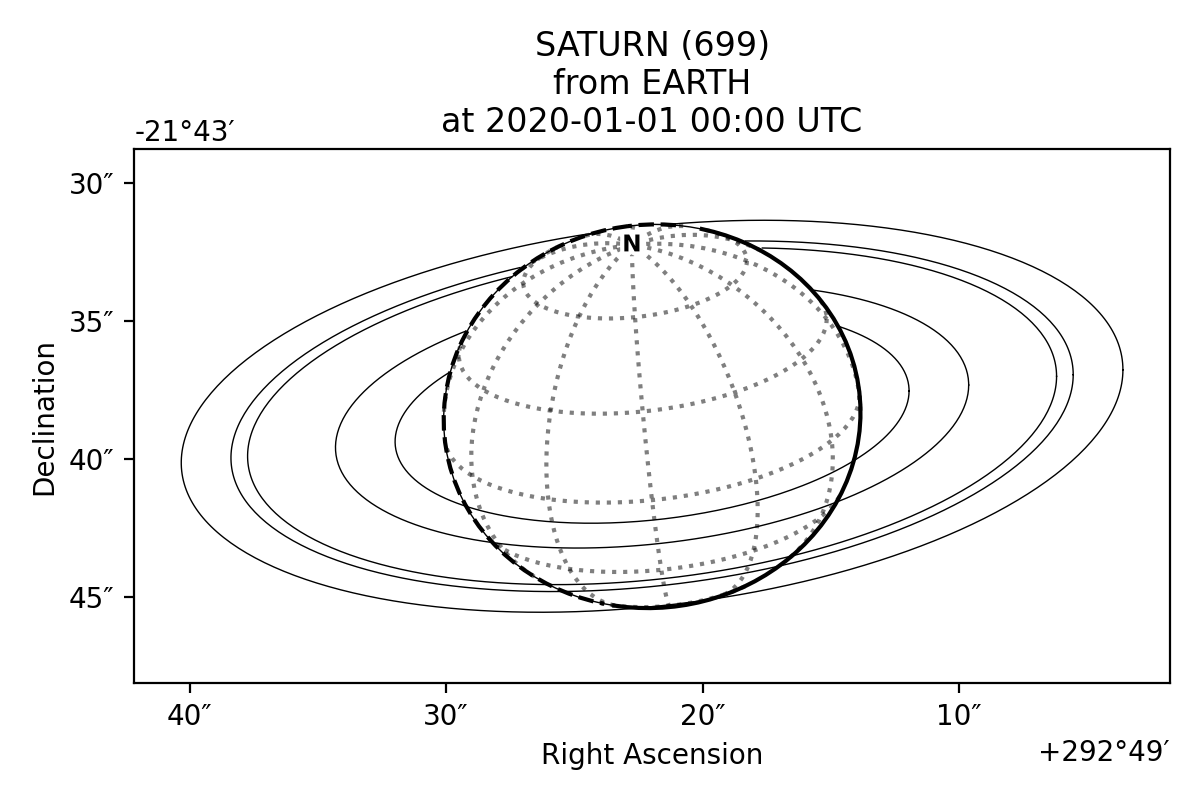
Wireframe plots

‘Wireframe’ plots showing the geometry of target bodies can be created quickly and easily using the planetmapper.Body.plot_wireframe_radec() command:

import planetmapper

body = planetmapper.Body('saturn', '2020-01-01')
body.plot_wireframe_radec(show=True)

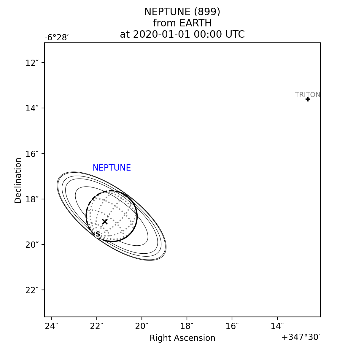
More complex plots can also be created using the functionality in planetmapper.Body and manually adding elements to the plot:

import planetmapper
import matplotlib.pyplot as plt

body = planetmapper.Body('neptune', '2020-01-01')

# Add Triton to any wireframe plots
body.add_other_bodies_of_interest('triton')

# Mark this specific coordinate (if visible) on any wireframe plots
body.coordinates_of_interest_lonlat.append((360, -45))

# Add Neptune's rings to the plot
body.add_named_rings()

fig, ax = plt.subplots(figsize=(6, 6), dpi=200)
body.plot_wireframe_radec(ax)

# Manually add some text to the plot
ax.text(
    body.target_ra, body.target_dec + 2 / 60 / 60, 'NEPTUNE', color='b', ha='center'
)

plt.show()

Wireframe plot variants

A number of different wireframe plotting options are available:

• planetmapper.Body.plot_wireframe_radec() plots in RA/Dec coordinates

• planetmapper.Body.plot_wireframe_km() plots in a frame centred showing distances in km from the target body

• planetmapper.Body.plot_wireframe_angular() plots in a frame showing angular distances from the the target body

• planetmapper.BodyXY.plot_wireframe_xy() plots in image x and y coordinates

• planetmapper.Body.plot_wireframe_custom() plots in a custom, user-defined, coordinate system

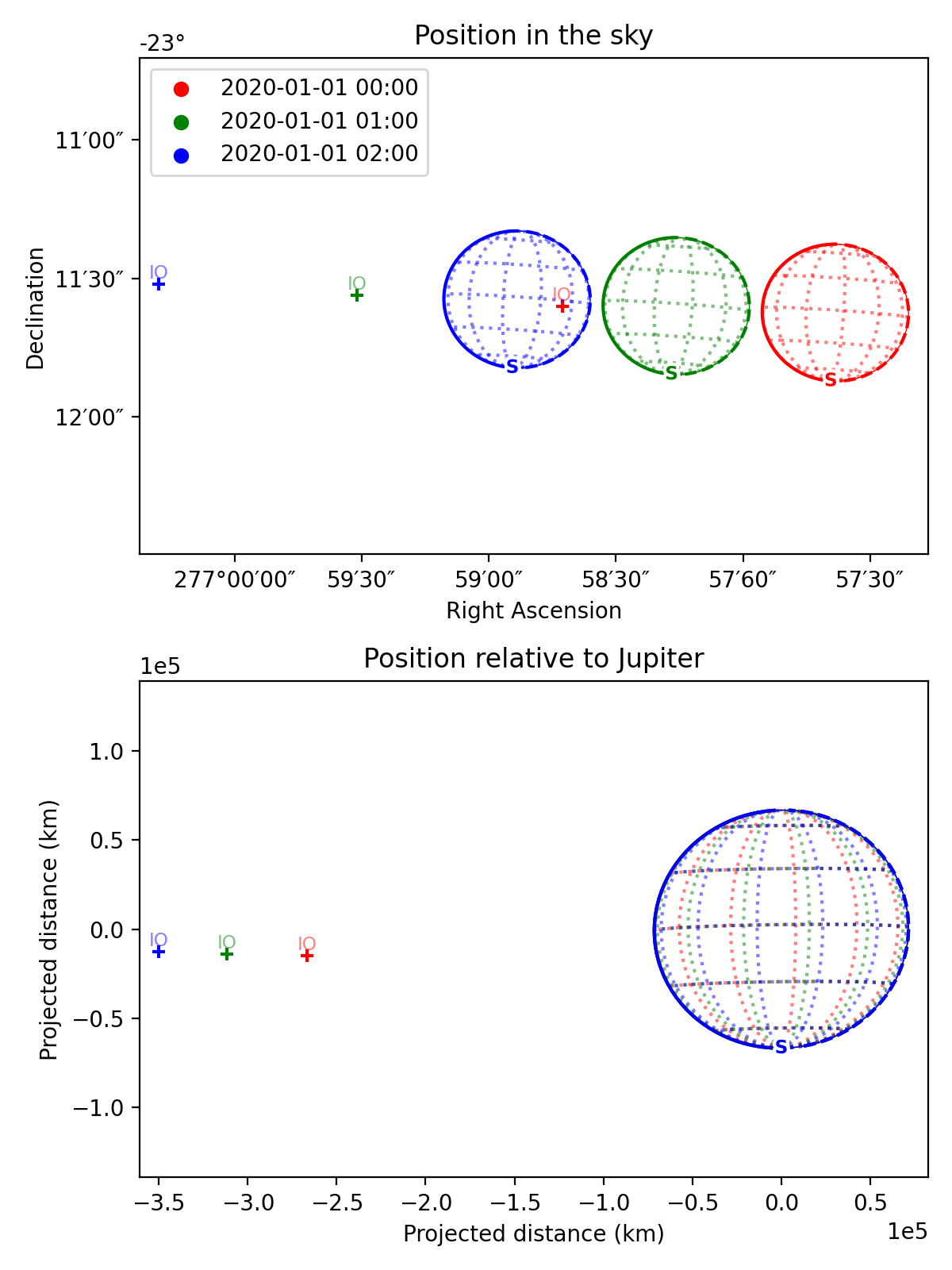
planetmapper.Body.plot_wireframe_km() is particularly useful for comparing observations taken at different times, as it standardises the position, orientation and size of the target body. The example below shows multiple observations of Jupiter and Io taken over the space of a few hours. Jupiter moves across the the RA/Dec plot (top), but stays fixed in the km plot (bottom), making it easier to see the relative motion of Io:

import planetmapper
import matplotlib.pyplot as plt
import numpy as np

fig, [ax_radec, ax_km] = plt.subplots(nrows=2, figsize=(6, 8), dpi=200)

dates = ['2020-01-01 00:00', '2020-01-01 01:00', '2020-01-01 02:00']
colors = ['r', 'g', 'b']

for date, c in zip(dates, colors):
    body = planetmapper.Body('jupiter', date)
    body.add_other_bodies_of_interest('Io')
    body.plot_wireframe_radec(ax_radec, color=c)
    body.plot_wireframe_km(ax_km, color=c)

    # Plot some blank data with the correct colour to go on the legend
    ax_radec.scatter(np.nan, np.nan, color=c, label=date)

ax_radec.legend(loc='upper left')

ax_radec.set_title('Position in the sky')
ax_km.set_title('Position relative to Jupiter')

fig.tight_layout()
plt.show()

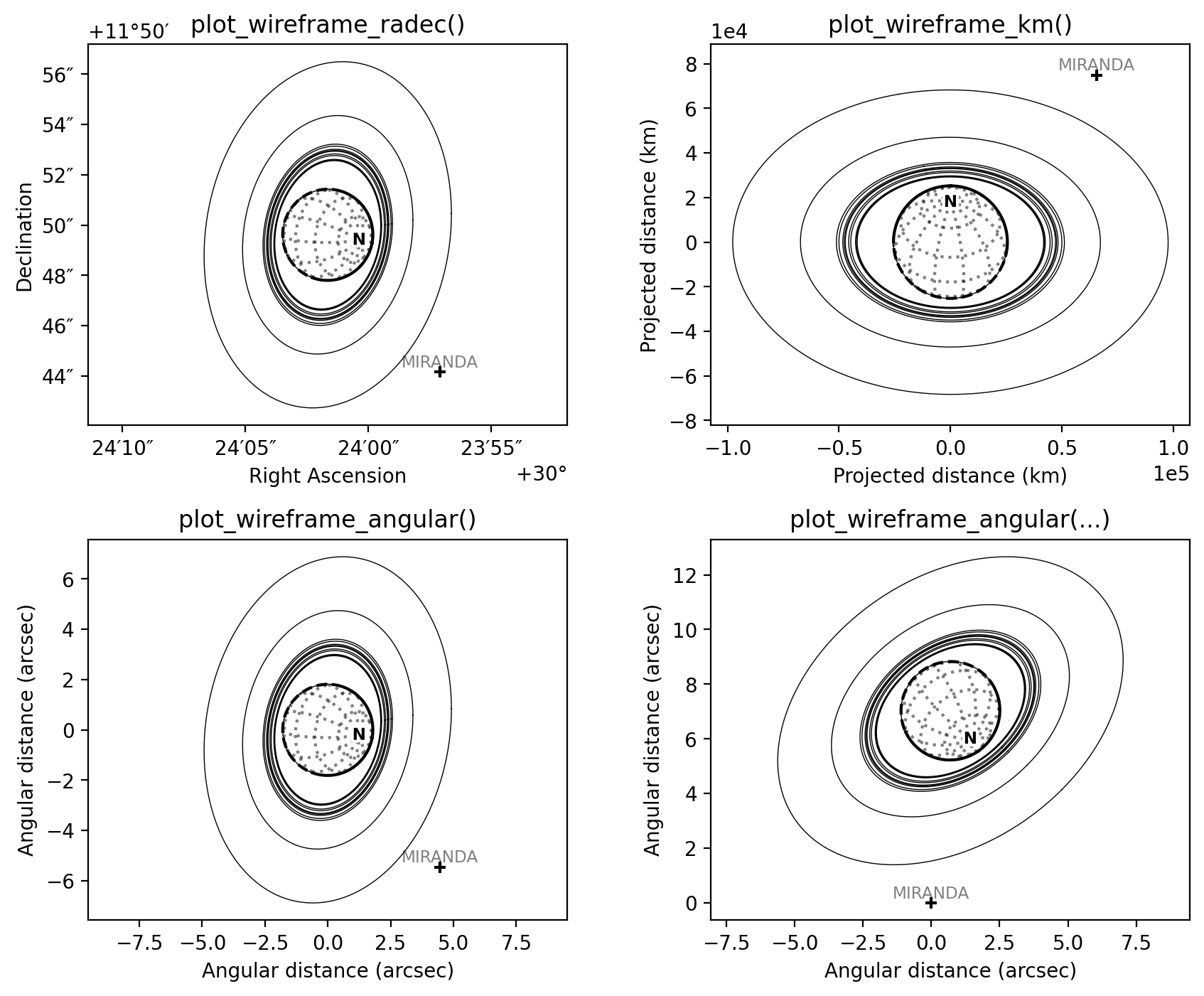
The example below shows how the the same target appears in the radec, km and angular wireframe variants. By default, planetmapper.Body.plot_wireframe_angular() is centred on the target body, but it can also be customised to have a custom origin and rotation - for example, the fourth plot below is centred on Miranda and rotated by 45°. In addition to the variants shown here, planetmapper.BodyXY.plot_wireframe_xy() is also available for use with planetmapper.BodyXY objects to plot in image pixel coordinates (see the Observations section below).

import planetmapper
import matplotlib.pyplot as plt

body = planetmapper.Body('uranus', '2020-01-01')
body.add_named_rings()
body.add_other_bodies_of_interest('miranda')

fig, ((ax_radec, ax_km), (ax_angular1, ax_angular2)) = plt.subplots(
    nrows=2,
    ncols=2,
    figsize=(10, 8),
    dpi=200,
    gridspec_kw=dict(hspace=0.3, wspace=0.3),
)

body.plot_wireframe_radec(ax_radec)
ax_radec.set_title('plot_wireframe_radec()')

body.plot_wireframe_km(ax_km)
ax_km.set_title('plot_wireframe_km()')

body.plot_wireframe_angular(ax_angular1)
ax_angular1.set_title('plot_wireframe_angular()')

miranda = body.create_other_body('miranda')
# angular plot centred on custom RA/Dec and with a custom rotation
body.plot_wireframe_angular(
    ax_angular2,
    origin_ra=miranda.target_ra,
    origin_dec=miranda.target_dec,
    coordinate_rotation=-45,
)
ax_angular2.set_title('plot_wireframe_angular(...)')

plt.show()

Customising wireframe plots

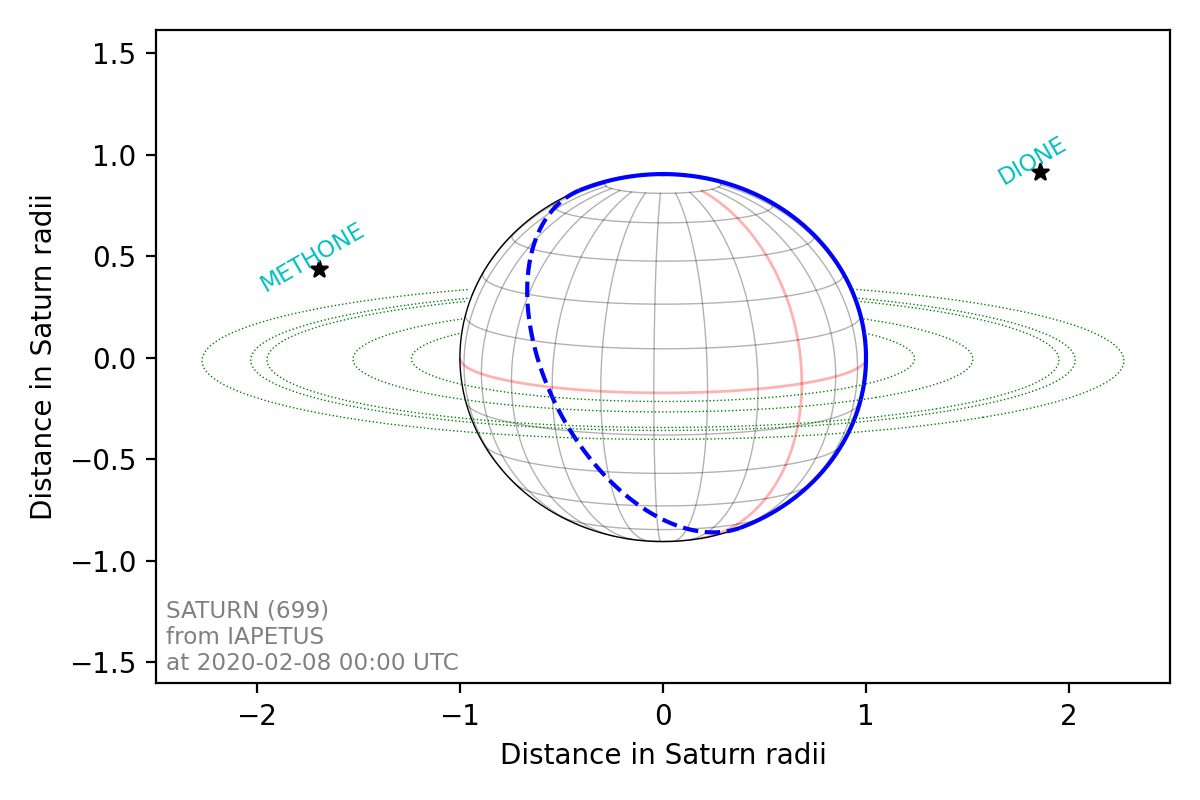
The appearance and units of wireframe plots can be fully customised to suit your needs. For example, the code below shows how the scale_factor argument is used to customise the coordinate units, and the formatting argument is used to pass arguments to matplotlib when plotting the individual elements of the wireframe. See planetmapper.Body.plot_wireframe_radec() for more details on formatting individual plots, and changing the default formatting for all wireframe plots.

import planetmapper
import matplotlib.pyplot as plt

body = planetmapper.Body('saturn', '2020-02-08', observer='iapetus')
body.add_other_bodies_of_interest('dione', 'methone')
body.plot_wireframe_km(
    ax,
    scale_factor=1 / body.r_eq,  # use units of Saturn radii rather than km
    add_title=False,
    label_poles=False,
    indicate_equator=True,
    indicate_prime_meridian=True,
    grid_interval=15,
    grid_lat_limit=75,
    formatting={
        'grid': {'linestyle': '-', 'linewidth': 0.5, 'alpha': 0.3},
        'prime_meridian': {'linewidth': 1, 'color': 'r'},
        'equator': {'linewidth': 1, 'color': 'r'},
        'terminator': {'color': 'b'},
        'limb_illuminated': {'color': 'b'},
        'ring': {'color': 'g', 'linestyle': ':'},
        'other_body_of_interest_marker': {'marker': '*'},
        'other_body_of_interest_label': {'color': 'c', 'rotation': 30, 'alpha': 1},
    },
)
ax.set_xlabel('Distance in Saturn radii')
ax.set_ylabel('Distance in Saturn radii')
ax.annotate(
    body.get_description(),
    (0.01, 0.02),
    xycoords='axes fraction',
    color='0.5',
    size='small',
)
plt.show()

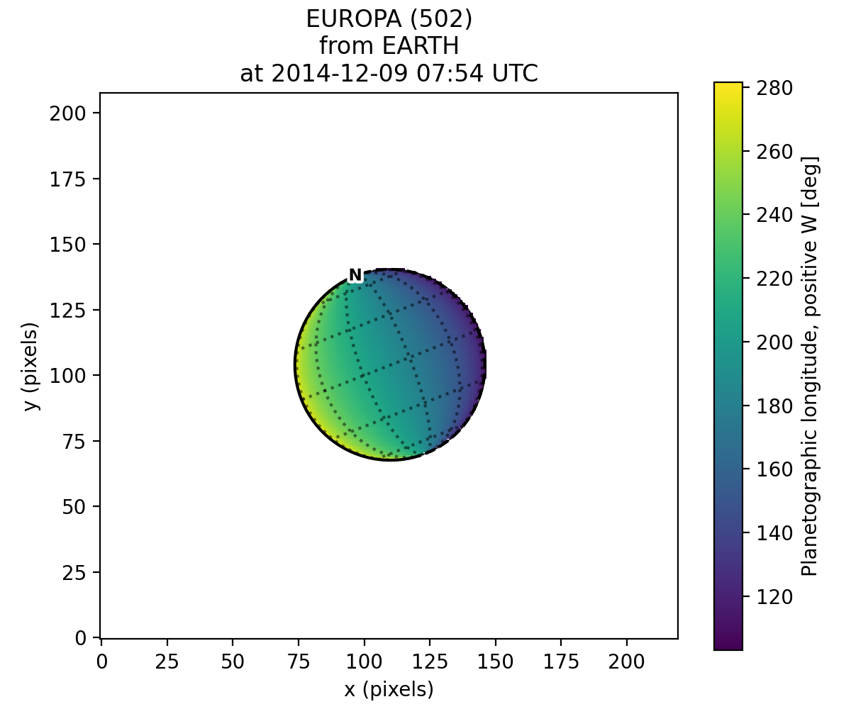
Observations, backplanes and mapping

Note

You can download an example Europa data file from the PlanetMapper GitHub repository.

planetmapper.Observation objects can be created to calculate information about a specific observation. If the observed data is saved in a FITS file with appropriate header information, a planetmapper.Observation object can be created using only the path to that file - target, date and observer information can all be derived automatically from the header. The example below creates an Observation object, and uses it to plot an image containing showing the longitude value of each pixel:

import planetmapper
import matplotlib.pyplot as plt

observation = planetmapper.Observation('europa.fits')

# Set the disc position
observation.set_plate_scale_arcsec(12.25e-3)
observation.set_disc_params(x0=110, y0=104)

observation.plot_backplane_img('LON-GRAPHIC')
plt.show()

A range of backplane images can be generated - see Default backplanes for a list of the backplanes available by default. These backplanes can be saved to a FITS file for future use using planetmapper.Observation.save_observation(). A mapped version of the image and backplanes can likewise be saved using planetmapper.Observation.save_mapped_observation():

import planetmapper

observation = planetmapper.Observation('europa.fits')

# Set the disc position
observation.set_plate_scale_arcsec(12.25e-3)
observation.set_disc_params(x0=110, y0=104)

observation.save_observation('europa_navigated.fits')
observation.save_mapped_observation('europa_mapped.fits')

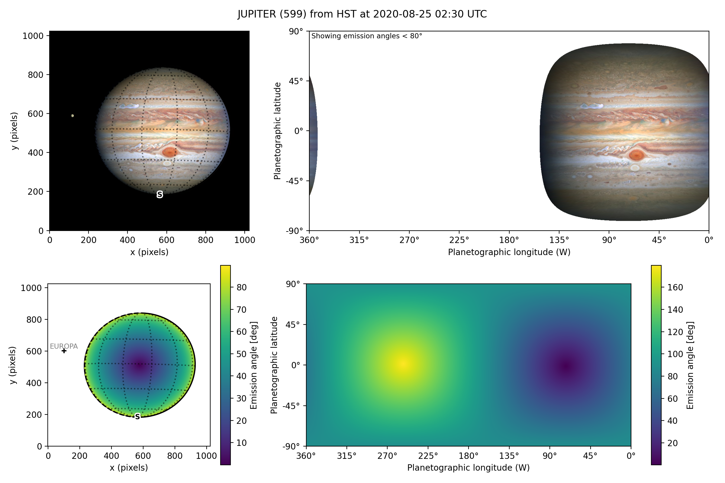
Mapped data can also be manipulated and plotted directly. In the example below, we use planetmapper.Observation.get_mapped_data() and planetmapper.BodyXY.get_backplane_map() to directly access, manipulate and plot the mapped data and backplanes:[1]

import planetmapper
import matplotlib.pyplot as plt
import numpy as np

# This uses a JPG image, so we need to manually specify details (e.g. target)
observation = planetmapper.Observation(
    'jupiter.jpg',
    target='jupiter',
    utc='2020-08-25 02:30:40',
    observer='HST',
    show_progress=True, # show progress bars for slower functions
)

# Run the GUI to fit the disc interactively
observation.run_gui()

fig, axs = plt.subplots(
    nrows=2, ncols=2, figsize=(12, 8), dpi=200, width_ratios=[1, 2]
)

# Do a nice RGB plot of the data in the top left
rgb_img = np.moveaxis(observation.data, 0, 2)  # imshow needs wavelength index last
axs[0, 0].imshow(rgb_img, origin='lower')
observation.plot_wireframe_xy(axs[0, 0])

# Plot the emission angle backplane in the bottom left
observation.add_other_bodies_of_interest('Europa')  # mark Europa on this plot
observation.plot_backplane_img('EMISSION', ax=axs[1, 0])

# Plot the mapped emission angle backplane in the bottom right
observation.plot_backplane_map('EMISSION', ax=axs[1, 1])


# Plot a mapped RGB image of the data in the top right
degree_interval = 0.25  # Plot maps with 4 pixels/degree
emission_cutoff = 80

mapped_data = observation.get_mapped_data(degree_interval)  # get the mapped data
rgb_map = np.moveaxis(mapped_data, 0, 2)  # imshow needs wavelength index last
rgb_map = planetmapper.utils.normalise(rgb_map)  # normalise to make plot look nicer

# Only plot areas with emission angles <80deg
emission_map = observation.get_backplane_map('EMISSION', degree_interval)
for idx in range(3):
    rgb_map[:, :, idx][np.where(emission_map > emission_cutoff)] = 1

# Display mapped image and add a useful annotation
observation.imshow_map(rgb_map, ax=axs[0, 1])
axs[0, 1].annotate(
    f'Showing emission angles < {emission_cutoff}°',
    (0.005, 0.99),
    xycoords='axes fraction',
    size='small',
    va='top',
)


# Add some general formatting
for ax in axs.ravel():
    ax.set_title('')
fig.suptitle(observation.get_description(multiline=False))
fig.tight_layout()

plt.show()

[1]

The Jupiter image is from the OPAL program using the Hubble Space Telescope. Credit: NASA, ESA, STScI, A. Simon (Goddard Space Flight Center), and M.H. Wong (University of California, Berkeley) and the OPAL team

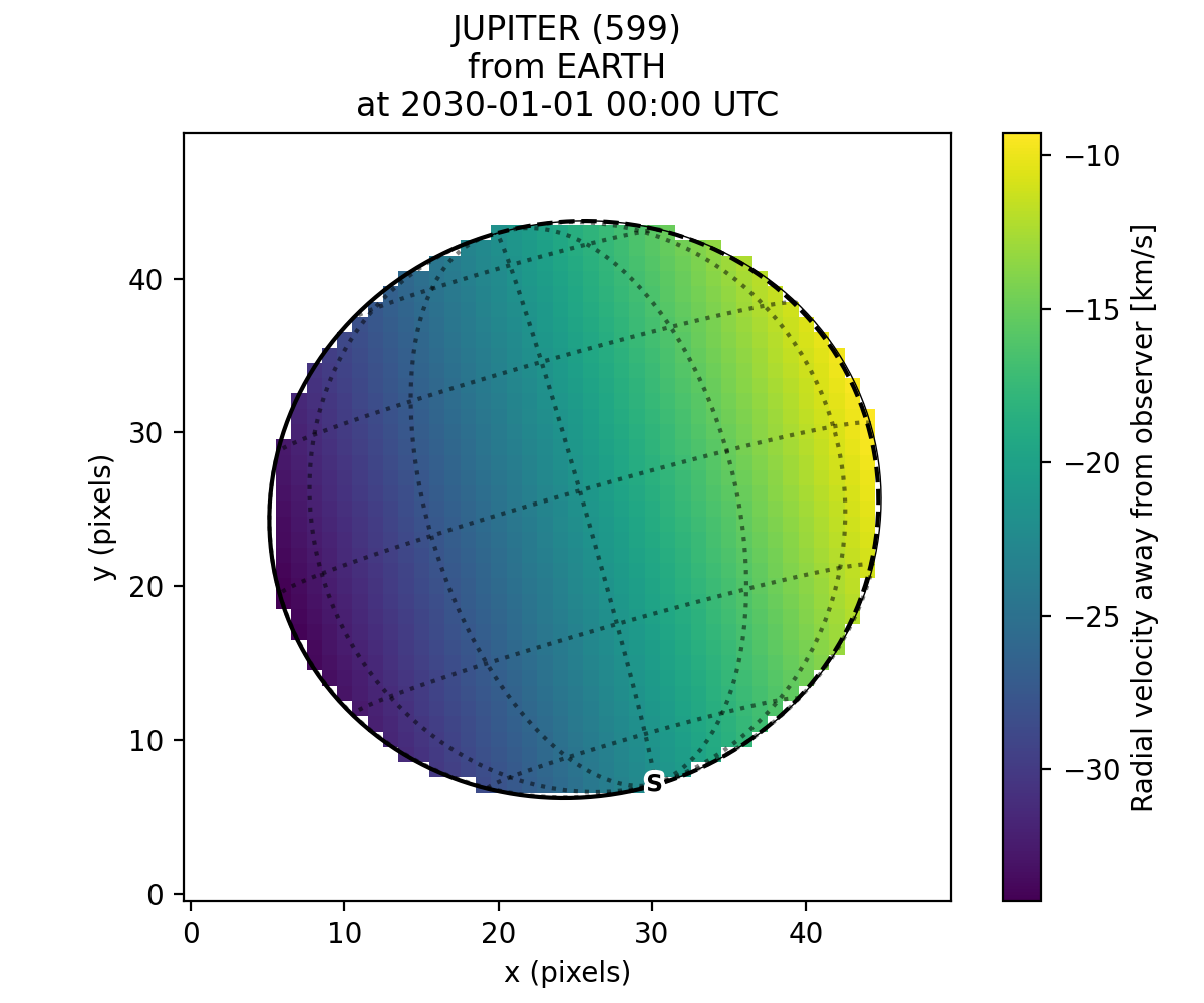
Backplanes can also be generated for observations which do not exist using planetmapper.BodyXY:

import planetmapper
import matplotlib.pyplot as plt
import numpy as np

# Create an object representing how Jupiter would appear in a 50x50 pixel image
# taken from Earth at a specific time
body = planetmapper.BodyXY('jupiter', utc='2030-01-01', observer='Earth', sz=50)
body.set_disc_params(x0=25, y0=25, r0=20)

fig, ax = plt.subplots(figsize=(6, 5), dpi=200)
body.plot_backplane_img('RADIAL-VELOCITY', ax=ax)
fig.tight_layout()
plt.show()

# Backplane images can also be accessed and manipulated directly
radial_velocities = body.get_backplane_img('RADIAL-VELOCITY')
print(f'Average radial velocity: {np.nanmean(radial_velocities):.2f} km/s')

# Average radial velocity: -21.78 km/s

Cache behaviour

The generation of backplanes and projected mapped data can be slow for larger datasets. Therefore, planetmapper.BodyXY and planetmapper.Observation objects automatically cache the results of various expensive function calls so that they do not have to be recalculated. This cache management happens automatically behind the scenes, so you should never have to worry about dealing with it directly. For example, when any disc parameters are changed, the cache is automatically cleared as the cached results will no longer be valid.

import planetmapper

# Create a new object
body = planetmapper.BodyXY('Jupiter', '2000-01-01', sz=500)
body.set_disc_params(x0=250, y0=250, r0=200)
# At this point, the cache is completely empty

# The intermediate results used in generating the incidence angle backplane
# are cached, speeding up any future calculations which use these
# intermediate results:
body.get_backplane_img('INCIDENCE') # Takes ~10s to execute
body.get_backplane_img('INCIDENCE') # Executes instantly
body.get_backplane_img('EMISSION') # Executes instantly

# When any of the disc parameters are changed, the xy <-> radec conversion
# changes so the cache is automatically cleared (as the cached intermediate
# results are no longer valid):
body.set_r0(190) # This automatically clears the cache
body.get_backplane_img('EMISSION') # Takes ~10s to execute
body.get_backplane_img('INCIDENCE') # Executes instantly

The methods which cache their results include…

• planetmapper.BodyXY.get_backplane_img()

• planetmapper.BodyXY.get_backplane_map()

• planetmapper.Observation.get_mapped_data()

• planetmapper.Observation.save_observation() and equivalent option in the GUI

• planetmapper.Observation.save_mapped_observation() and equivalent option in the GUI

Note

The Python script used to generate all the figures shown on this page can be found here